Demo 7: Using CAST to align the left and right hemispheres in the ARISTA Dataset
[1]:
%matplotlib widget
import CAST
import os,torch
import numpy as np
import anndata as ad
import scanpy as sc
import matplotlib.pyplot as plt
import warnings
from os.path import join as pj

warnings.filterwarnings('ignore')
plt.set_loglevel('ERROR')
os.environ['CUDA_LAUNCH_BLOCKING'] = '1'

# work_dir = '$demo_path' #### input the demo path
work_dir = "/home/unix/panj/wanglab/jessica/CAST/demo"
To demonstrate the CAST workflow on another dataset, we use CAST Mark and CAST Stack to align the left and right hemispheres of samples in the Axolotl Regenerative Telencephalon Interpretation via Spatiotemporal Transcriptomic Atlas (ARTISTA) (Wei et al., 2022).
This axolotl brain dataset contains coronal slices of the axolotl brain with experimentally introduced injuries on one hemisphere while the other hemisphere remained intact and healthy as the control at different days post injury (DPI) along the brain regeneration process.
For this demo, we demonstrate
CAST’s Interactive Widget
Use the widget to split a sample into its left (intact) and right (injured) hemispheres
CAST Alignment
Use CAST Mark to capture common spatial features between the two hemispheres
Use CAST Stack to align the two hemispheres to each other to help gain insights into the regeneration process
[2]:
### setting up output paths

task_name_t = '20231204artista_all_5k_half'

widget_outpath = pj(work_dir, 'demo7_ARTISTA/demo_output/artista_split_widget')
os.makedirs(widget_outpath, exist_ok=True)

mark_outpath  = pj(work_dir, 'demo7_ARTISTA/demo_output/artista_split_mark')
os.makedirs(pj(mark_outpath, "delaunay"), exist_ok=True)
os.makedirs(pj(mark_outpath, "kmeans_clustering"), exist_ok=True)

stack_outpath  = pj(work_dir, 'demo7_ARTISTA/demo_output/artista_split_stack')
os.makedirs(stack_outpath, exist_ok=True)
Splitting Samples With an Interactive Widget
[4]:
### load data
input_path = pj(work_dir, 'demo7_ARTISTA/data/artista_5k.h5ad')
adata = ad.read_h5ad(input_path)
coords_raw = adata.obsm['spatial'].copy()

### getting the data for a specific sample (2DPI_3)
slice_t = '2DPI_3'
idx_t = adata.obs['sample'] == slice_t
coords_one_slice = coords_raw[idx_t]
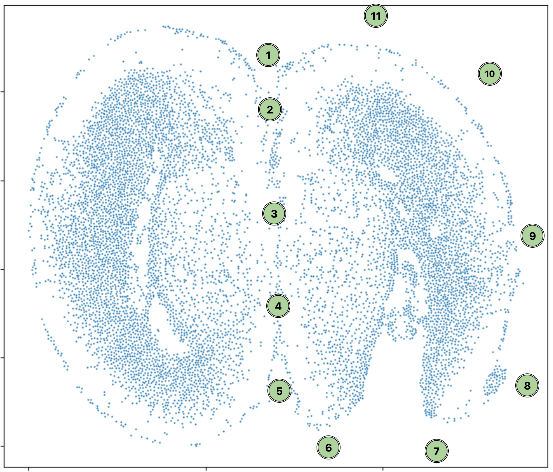
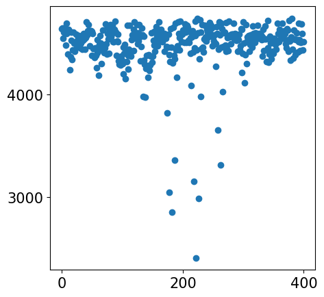
Here, we demonstrate CAST’s interactive widget for splitting a sample into two batches based on user-selected polygons.
This widget provides an interactive interface where the user can define polygons to isolate regions of their sample, such as separating the left and right hemispheres of the ARISTA dataset. The polygons are used to create a bitmask, enabling the segregation of the data for alignment.
As an example, to select the right (injured) hemisphere of this sample, run the cell below and click on the points following the order indicated in the following screenshot. When you finish, click “Finish Polygon.” A list of selected cell IDs should appear below the widget. If at any point you’d like to reset, click “Clear Polygon.”
[ ]:
### The interactive widget

from CAST.utils import cell_select

CAST.cell_select(coords_one_slice, output_path_t=f'{widget_outpath}/selected_cells{slice_t}.png')
[ ]:
## Display the split hemispheres
from CAST.utils import selected_cell_ids
from CAST.visualize import plot_mid
### Isolate cells into the left and right hemispheres
idx_t = np.zeros(coords_one_slice.shape[0],dtype = bool)
right_half_idx = idx_t.copy()
right_half_idx[np.array(CAST.utils.selected_cell_ids,dtype = int)] = True
left_half_idx = ~right_half_idx #& idx_t_remain
torch.save([left_half_idx,right_half_idx],f'{widget_outpath}/{slice_t}left_right_half_idx.pt')
### Separate the hemispheres into injured and normal
sample_list = ['injured','normal']
coords = {}
for sample_t in sample_list:
coords[sample_t] = coords_one_slice[right_half_idx] if sample_t=='injured' else coords_one_slice[left_half_idx]
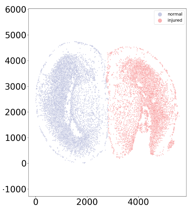
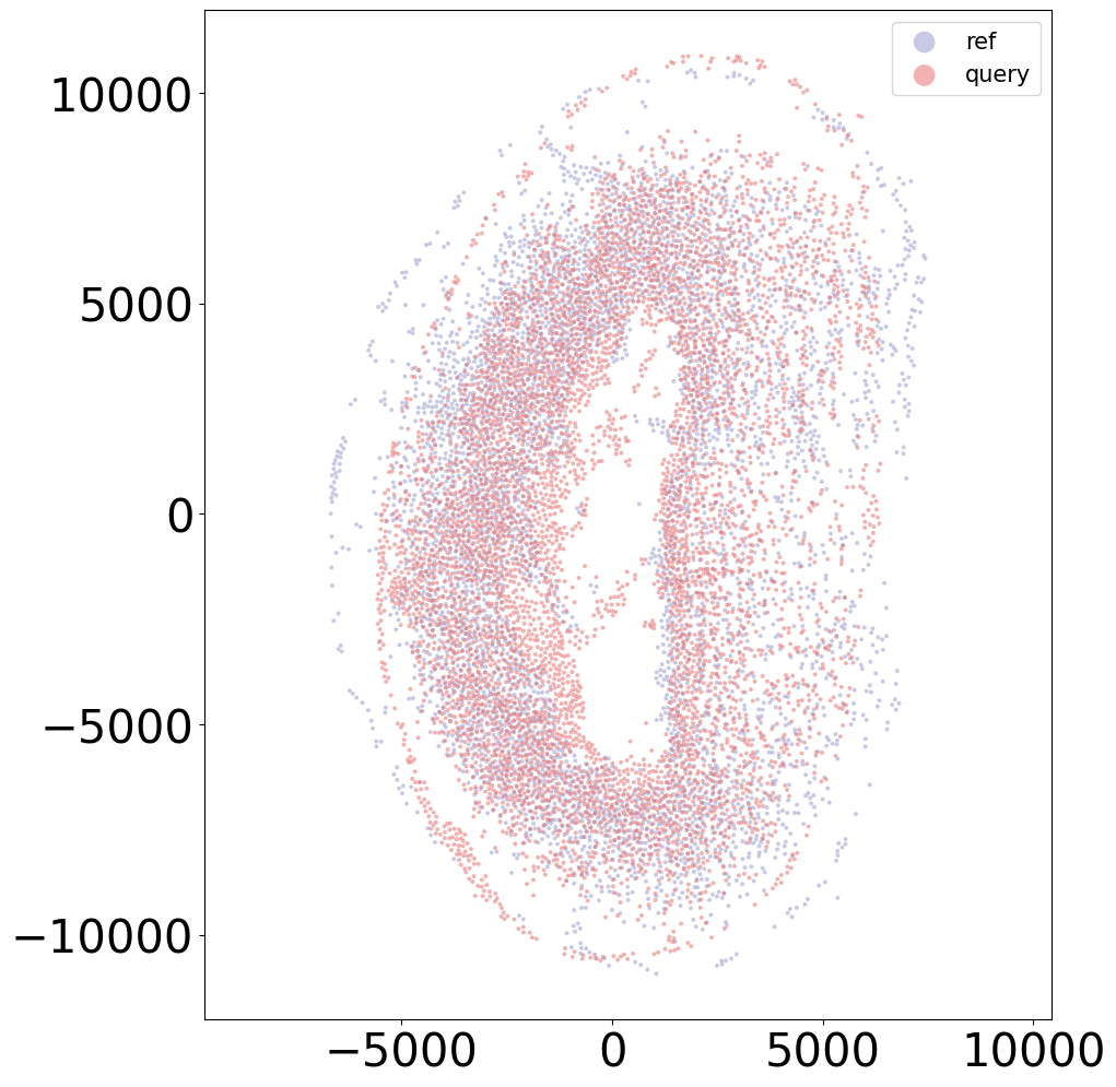
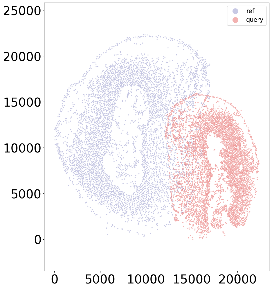
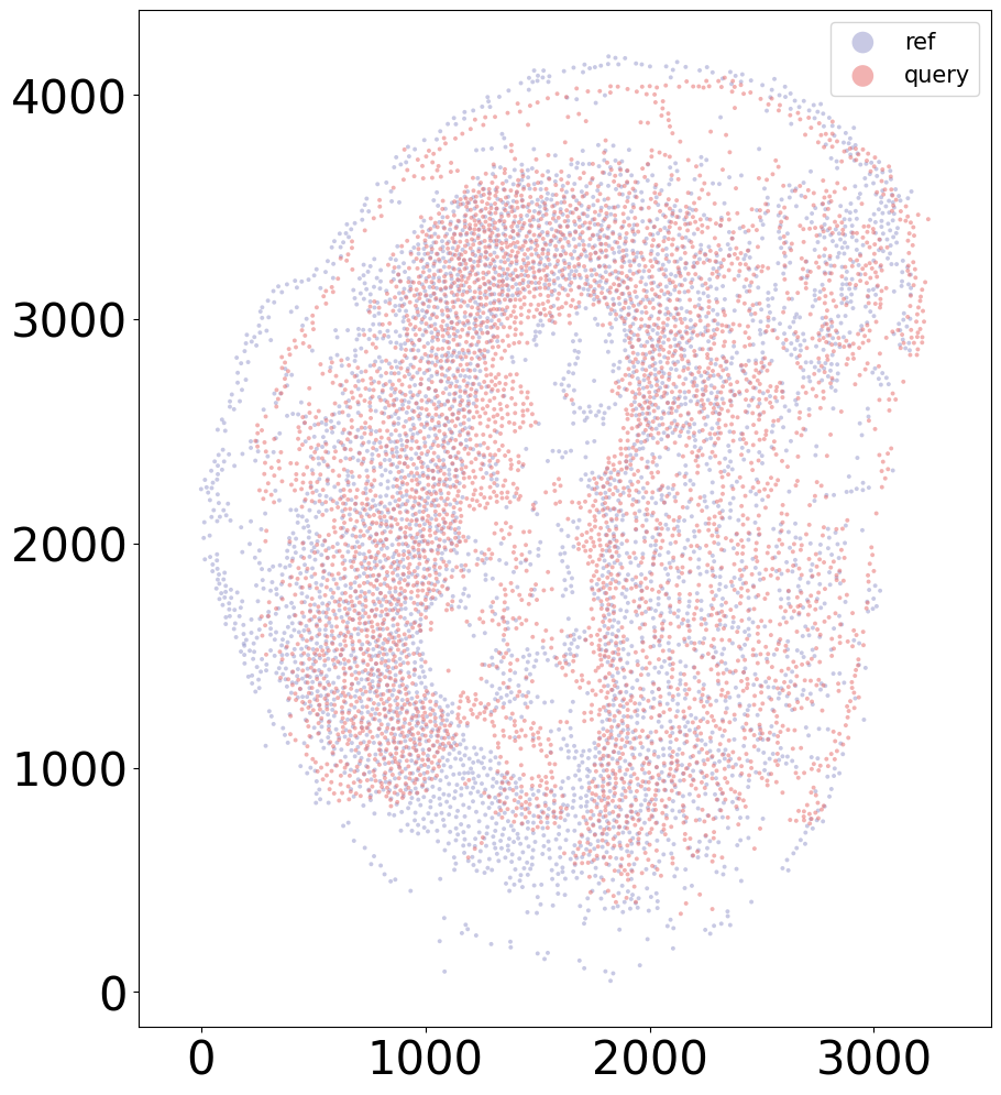
### Plot the two hemispheres
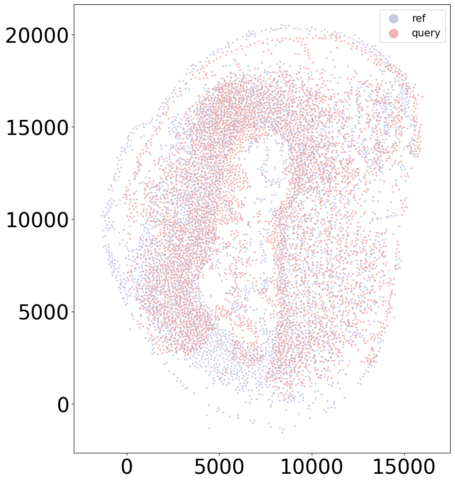
CAST.plot_mid(coords[sample_list[0]],
coords[sample_list[1]],
output_path=widget_outpath,
filename = f'{slice_t}_Align_raw',
title_t = [sample_list[1],
sample_list[0]],
s_t = 8,scale_bar_t = None)
Once you’ve selected the right hemisphere with the widget, the result should look like this:
Because this would be tedious to do for all 19 samples in the ARTISTA dataset, the rest of the samples have been pre-split.
CAST Mark
[5]:
### Initial setup (loading data)

adata = sc.read_h5ad(pj(work_dir, 'demo7_ARTISTA/data/artista_5k_half.h5ad'))
samples = np.unique(adata.obs['sample_half'])
adata.layers['norm1e4'] = sc.pp.normalize_total(adata, layer='counts', target_sum=1e4, inplace=False)['X']
exps_raw = {sample: adata[adata.obs['sample_half'] == sample].layers['norm1e4'].todense() for sample in samples}
coords_raw = {sample: adata[adata.obs['sample_half'] == sample].obsm['spatial'] for sample in samples}
[6]:
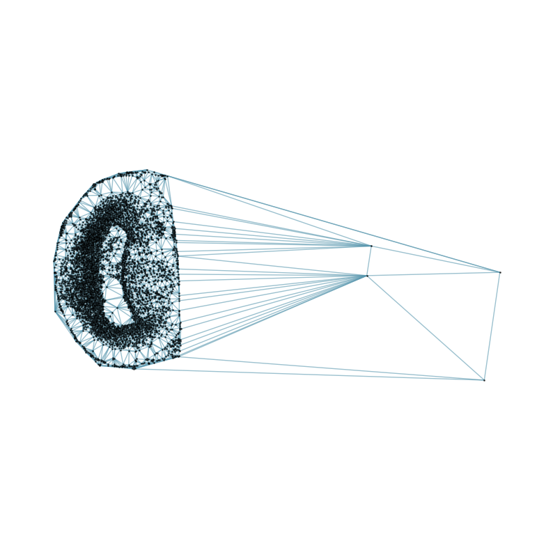
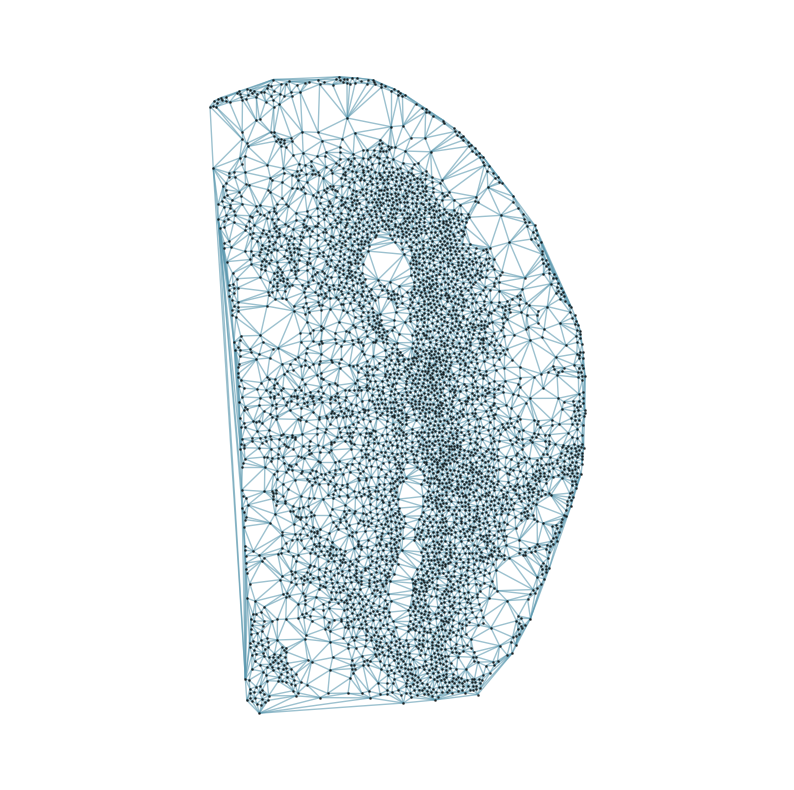
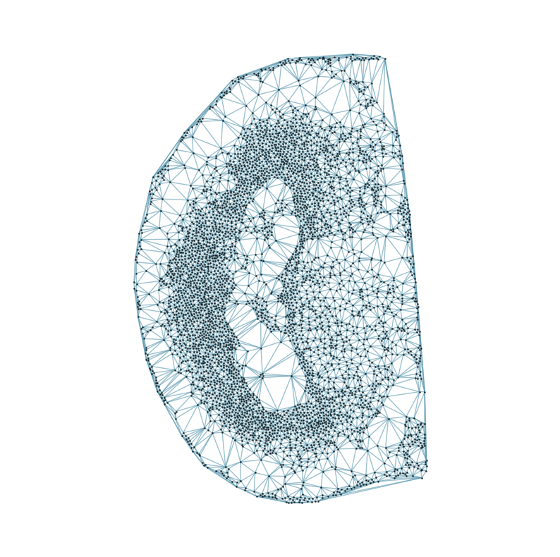
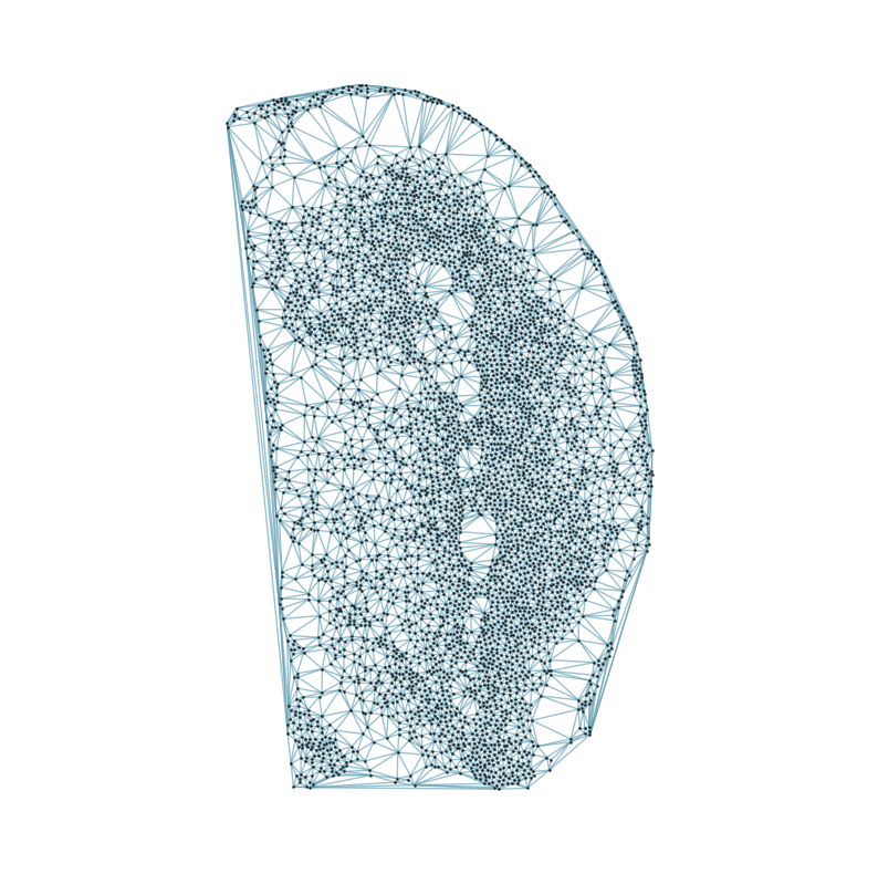
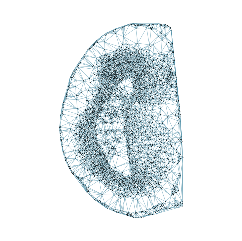
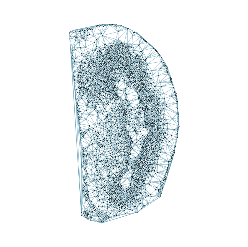
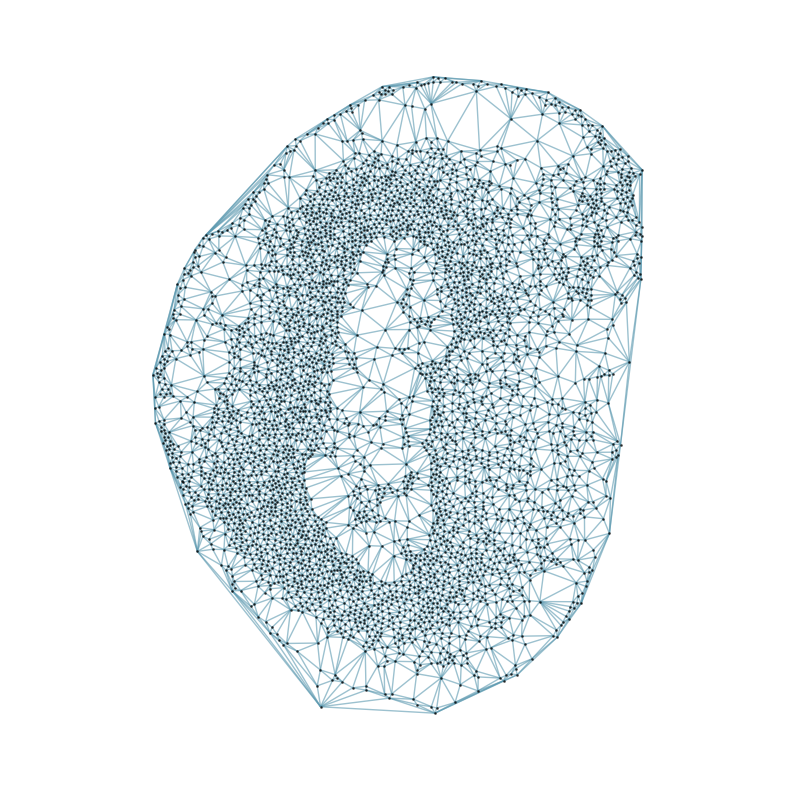
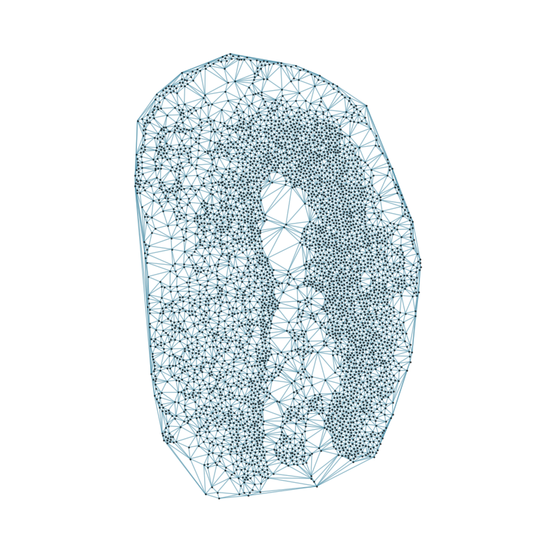
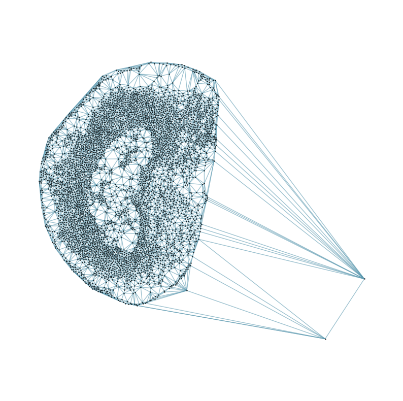
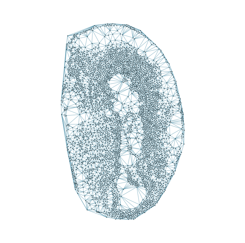
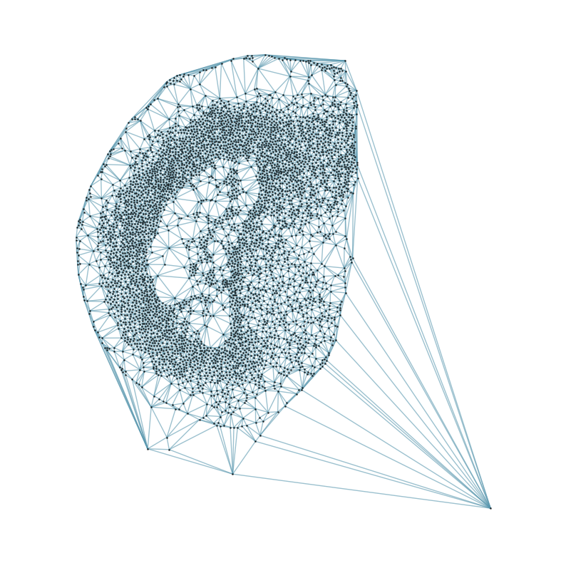
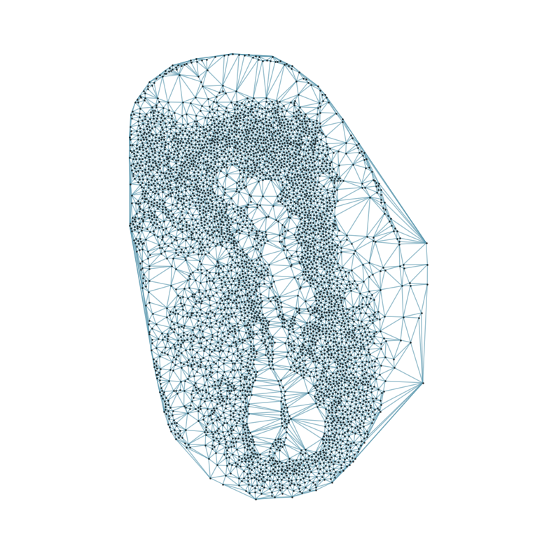
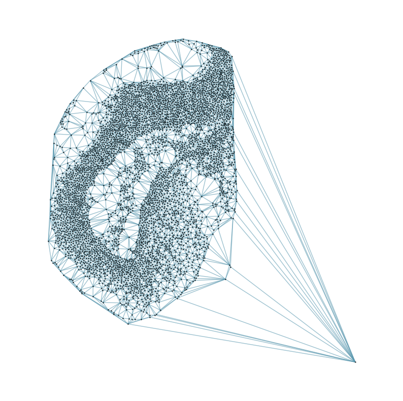
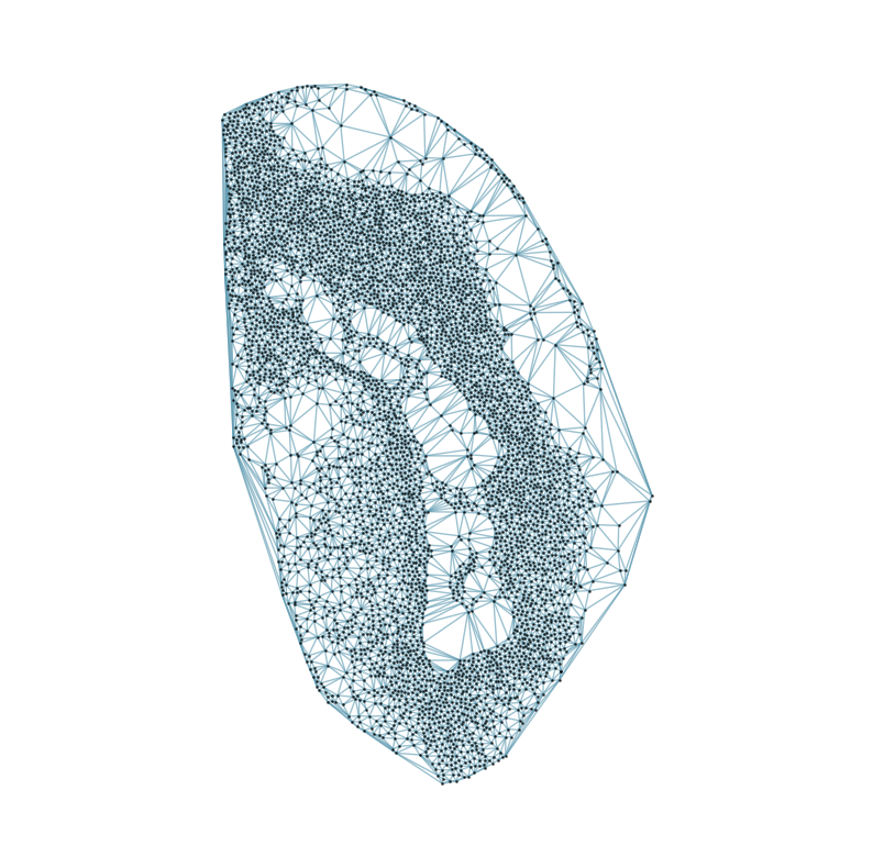
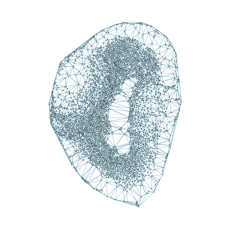
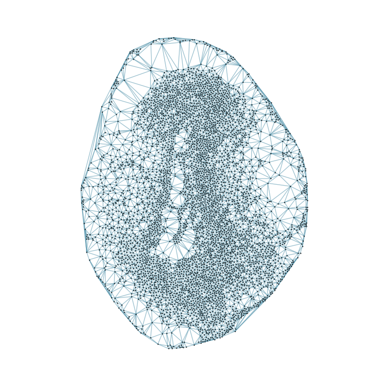
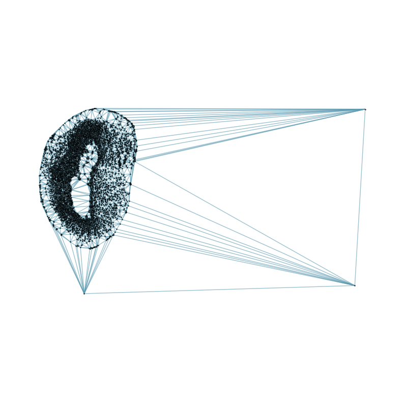
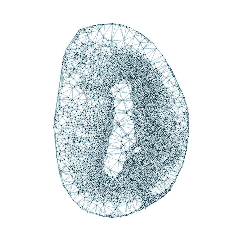
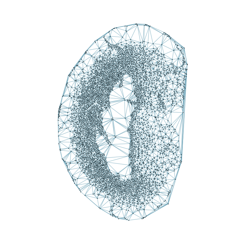
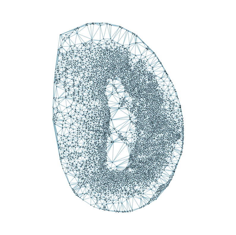
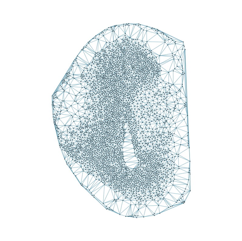
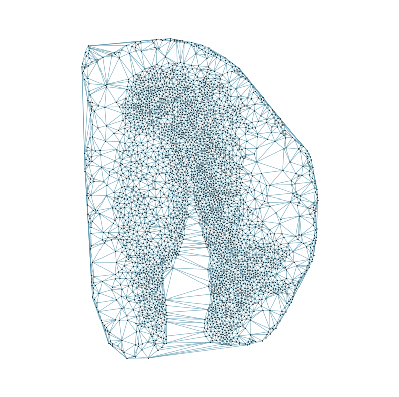
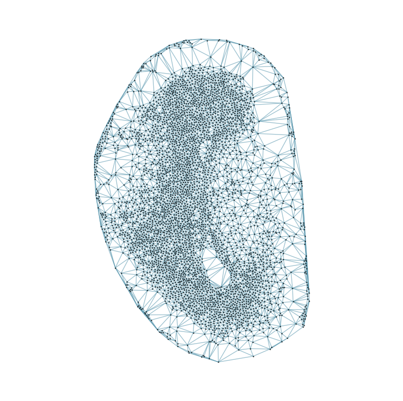
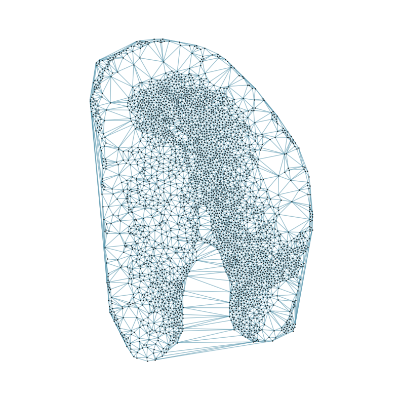
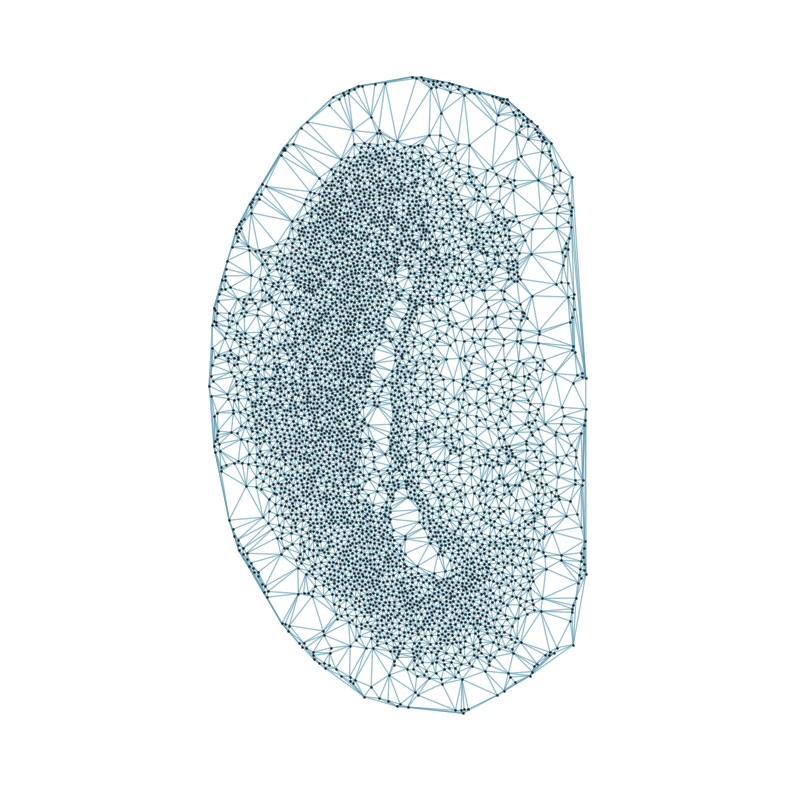
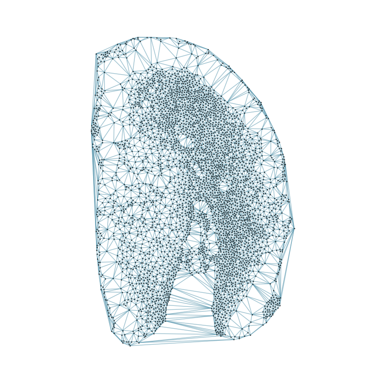
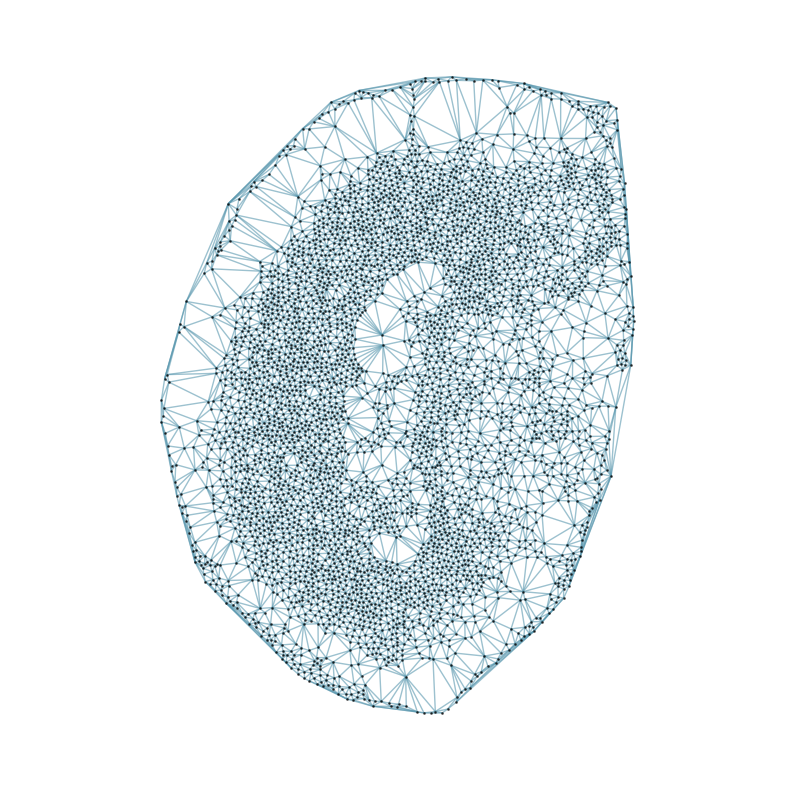
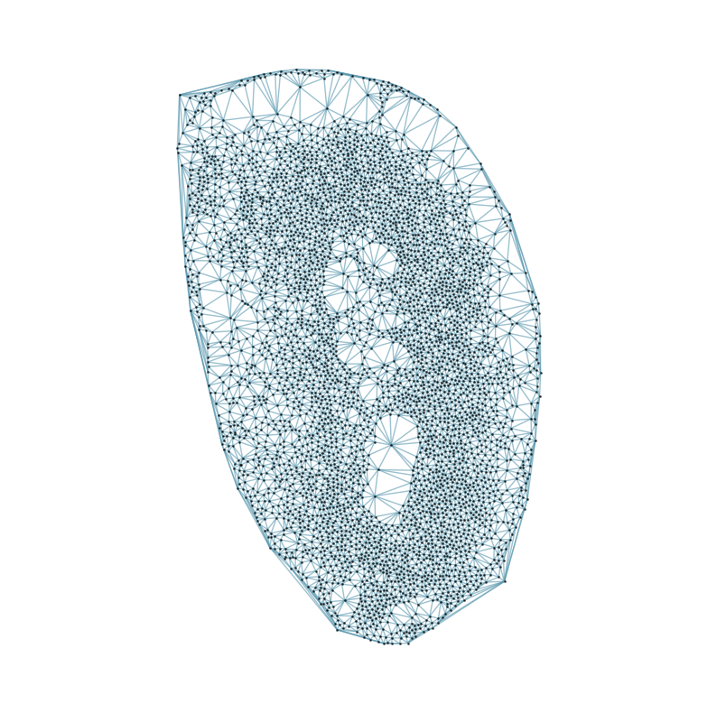
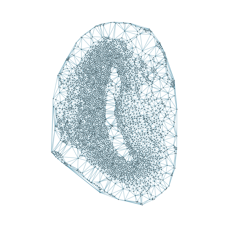
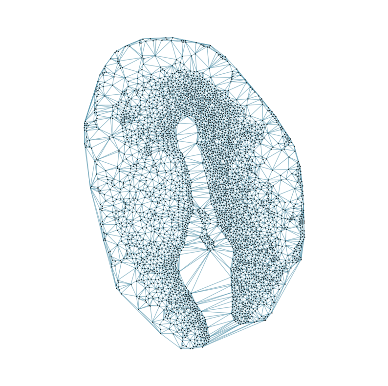
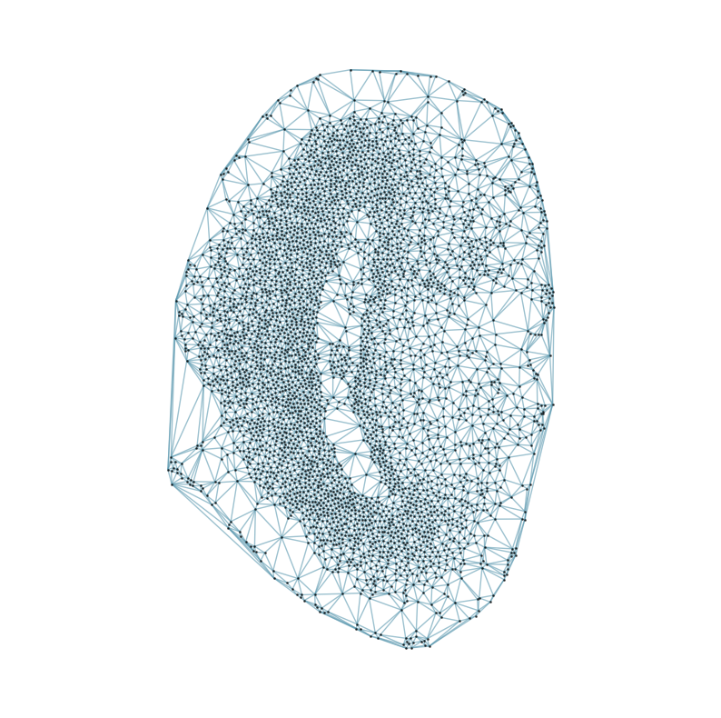
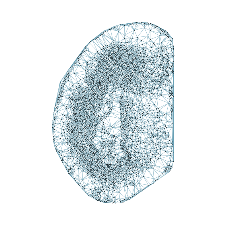
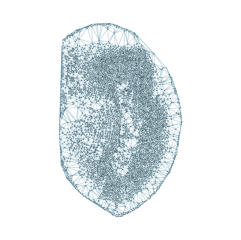
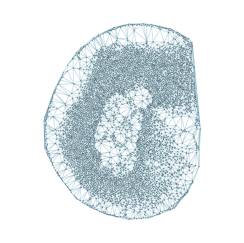
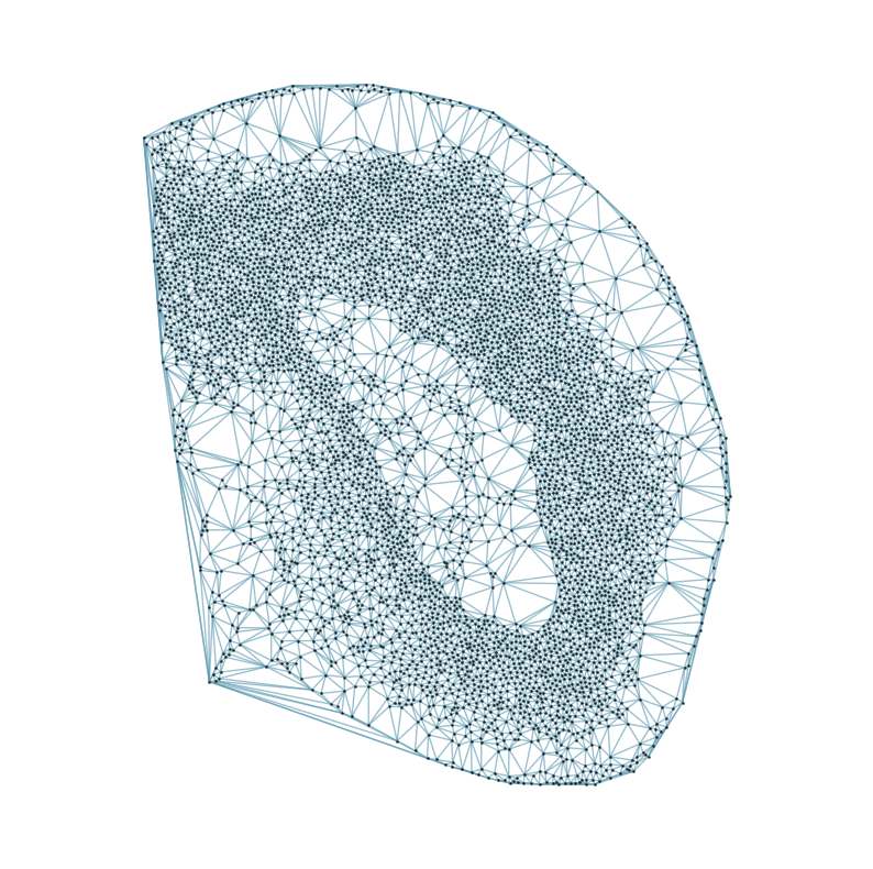
### Visualizing the delaunay graphs for all samples

from CAST.CAST_Mark import delaunay_dgl

device = 'cuda:0'
inputs = []

### construct delaunay graphs and input data
print(f'Constructing delaunay graphs for {len(samples)} samples...')
for sample_t in samples:
    graph_dgl_t = delaunay_dgl(sample_t,coords_raw[sample_t], pj(mark_outpath, "delaunay"), if_plot=True, strategy_t = 'delaunay').to(device)
    feat_torch_t = torch.tensor(exps_raw[sample_t], dtype=torch.float32, device=device)
    inputs.append((sample_t, graph_dgl_t, feat_torch_t))
Constructing delaunay graphs for 38 samples...
[7]:
### Initializing and trainng the GNN - this took ~70 minutes

from CAST.models.model_GCNII import CCA_SSG, Args
from CAST.CAST_Mark import train_seq

### parameters setting
args = Args(
    dataname=task_name_t + 'norm1e4_512', # name of the dataset, used to save the log file
    gpu = 0, # gpu id, set to zero for single-GPU nodes
    epochs=1500, # number of epochs for training
    lr1= 1e-3, # learning rate
    wd1= 0, # weight decay
    lambd= 1e-3, # lambda in the loss function, refer to online methods
    n_layers=9, # number of GCNII layers, more layers mean a deeper model, larger reception field, at a cost of VRAM usage and computation time
    der=0.5, # edge dropout rate in CCA-SSG
    dfr=0.3, # feature dropout rate in CCA-SSG
    use_encoder=True, # perform a single-layer dimension reduction before the GNNs, helps save VRAM and computation time if the gene panel is large
    encoder_dim=512, # encoder dimension, ignore if `use_encoder` set to `False`
)

### Initialize the model
in_dim = inputs[0][-1].size(-1)
model = CCA_SSG(in_dim=in_dim, encoder_dim=args.encoder_dim, n_layers=args.n_layers, use_encoder=args.use_encoder).to(args.device)

### Training
print(f'Training on {args.device}...')
embed_dict, loss_log, model = train_seq(graphs=inputs, args=args, dump_epoch_list=[], out_prefix=f'{mark_outpath}/{task_name_t}_seq_train', model=model)

### Saving the results
torch.save(embed_dict, f'{mark_outpath}/{args.dataname}_embed_dict.pt')
torch.save(loss_log, f'{mark_outpath}/{args.dataname}_loss_log.pt')
torch.save(model, f'{mark_outpath}/{args.dataname}_model_trained.pt')

### Plotting the loss
plt.plot(loss_log)
plt.title("Loss per Epoch")

print(f'Finished.')
print(f'The embedding, log, model files were saved to {mark_outpath}')
Training on cuda:0...
Loss: -263.685 step time=2.646s: 1%| | 10/1500 [00:28<1:07:31, 2.72s/it]Loss: -441.590 step time=2.706s: 100%|████| 1500/1500 [1:07:14<00:00, 2.69s/it]
Finished.
The embedding, log, model files were saved to /home/unix/panj/wanglab/jessica/CAST/demo/demo7_ARTISTA/demo_output/artista_split_mark

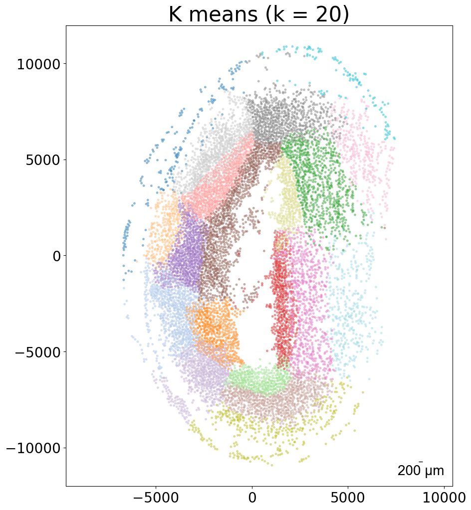
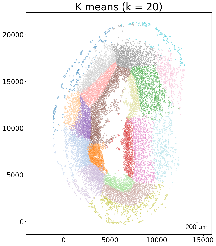
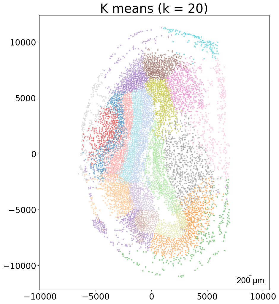
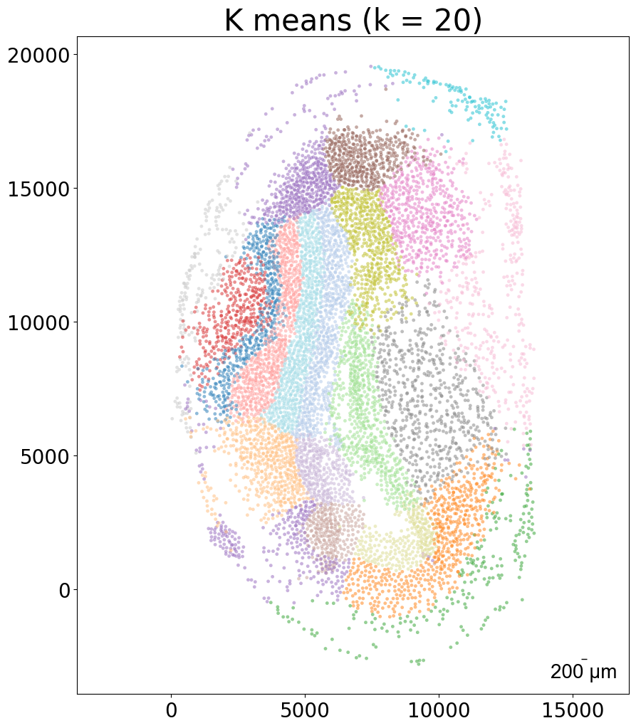
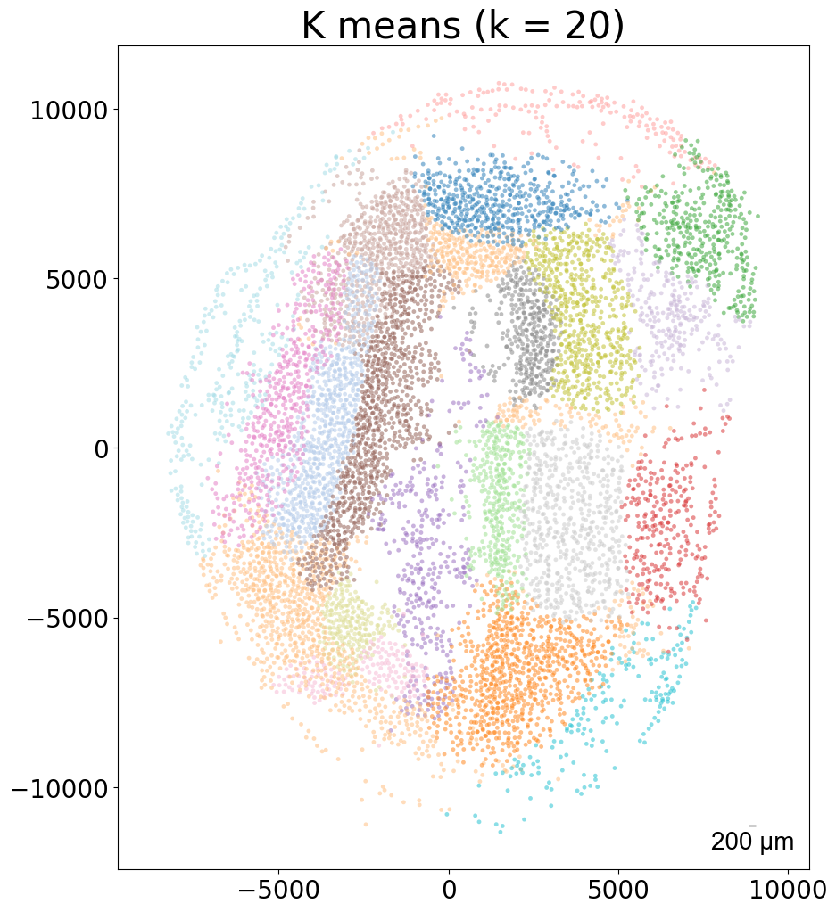
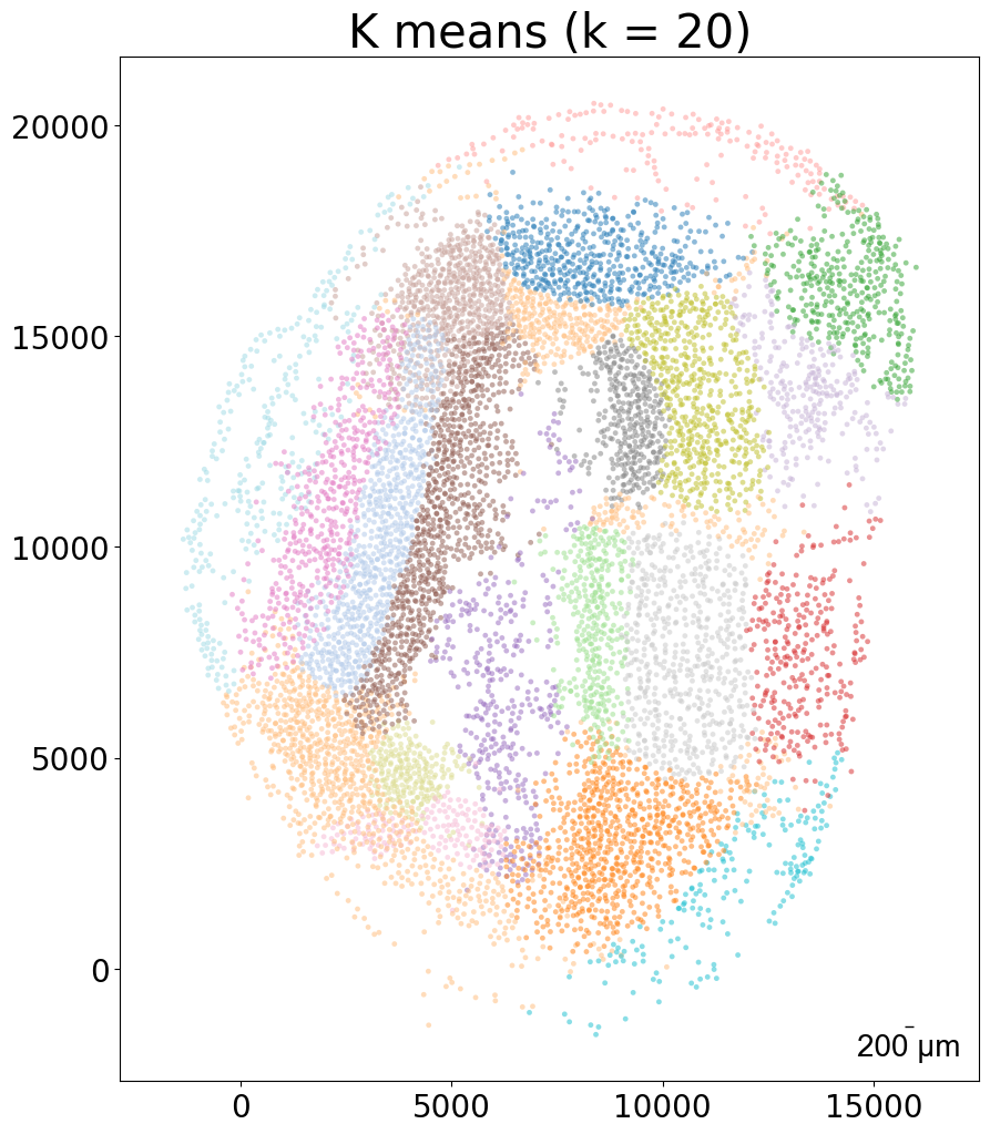
[8]:
### k-means clustering results per sample (k = 10)

from CAST import kmeans_plot_multiple

torch.load(f'{mark_outpath}/{args.dataname}_embed_dict.pt')
kmeans_plot_multiple(embed_dict, samples, coords_raw, args.dataname, pj(mark_outpath, "kmeans_clustering"), k = 10)
Perform KMeans clustering on 182142 cells...
Plotting the KMeans clustering results...
[8]:
array([8, 8, 8, ..., 9, 9, 9], dtype=int32)
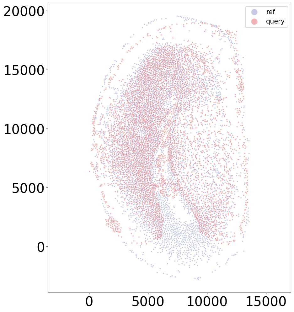
CAST Stack
[9]:
### Set up and load data

embed_dict = torch.load(f'{mark_outpath}/{task_name_t}norm1e4_512_embed_dict.pt') # from running CAST Mark
adata = sc.read_h5ad(pj(work_dir, 'demo7_ARTISTA/data/artista_5k_half.h5ad'))
coords_raw = {sample: adata[adata.obs['sample_half'] == sample].obsm['spatial'].copy() for sample in adata.obs['sample_half'].unique()}
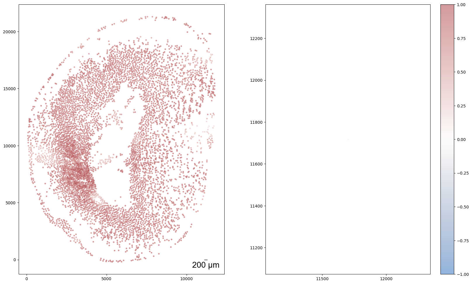
[10]:
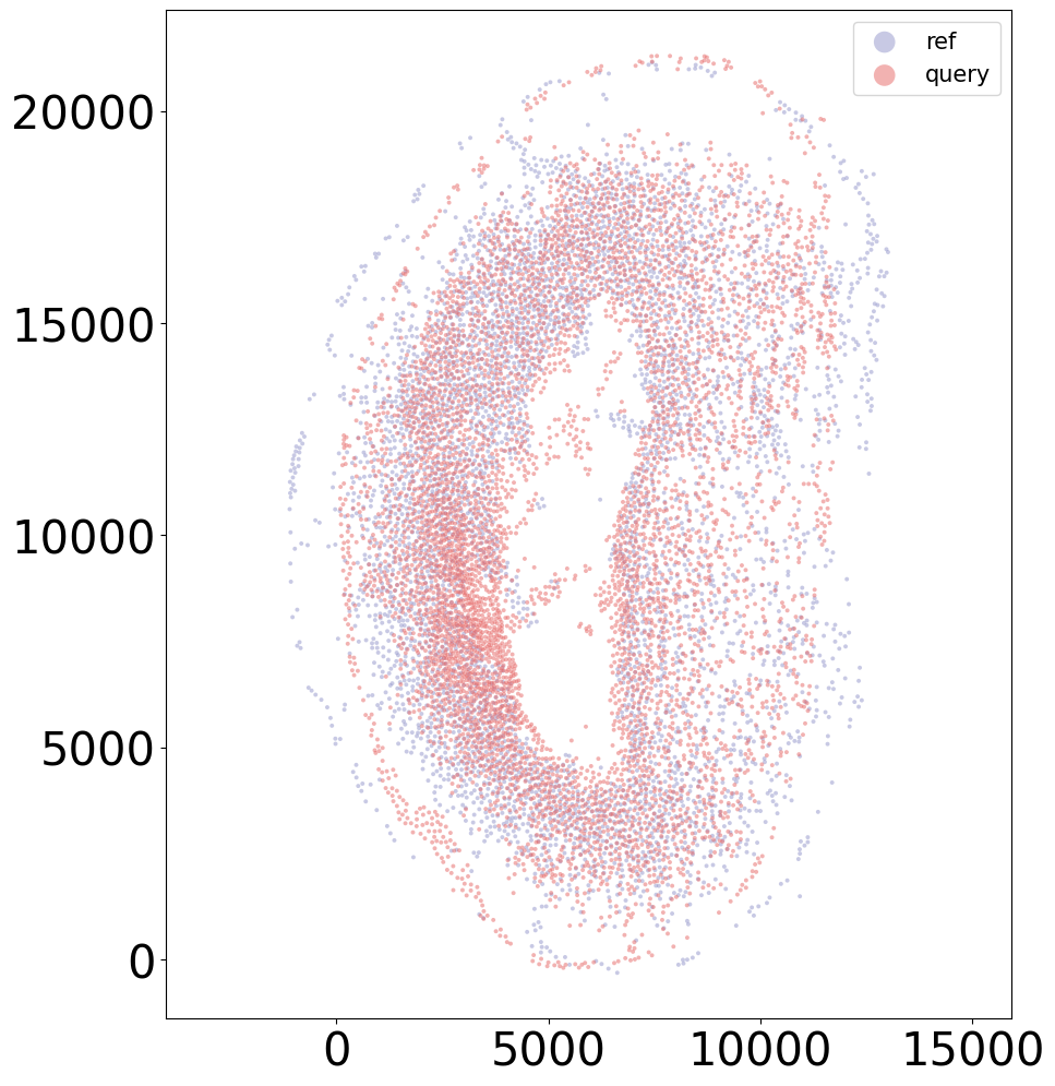
### define CAST Stack function with parameters
from CAST import reg_params, CAST_STACK
def align(reference_sample, query_sample, output_dataname):
"""Set up paramters and run CAST Stack, given the name of the reference and query samples, and the output folder name. """
graph_list = [query_sample, reference_sample]
### CAST Stack parameters -- see demo 2 for more information on these parameters
params_dist = reg_params(dataname = query_sample,
diff_step = 5,
gpu = 0 if torch.cuda.is_available() else -1,
#### Affine parameters
iterations=300,
dist_penalty1=0,
bleeding=500,
d_list = [1],
attention_params = [None,3,1,0],
translation_params = [0.5,0.5,10],
mirror_t = [-1],
#### FFD parameters
dist_penalty2 = [2],
alpha_basis_bs = [500],
meshsize = [8],
iterations_bs = [160],
attention_params_bs = [[None,3,1,0]],
mesh_weight = [None])
params_dist.alpha_basis = torch.Tensor([1/1000,1/1000,1/50,5,5]).reshape(5,1).to(params_dist.device)
### setting up output path
stack_outdir = pj(stack_outpath, output_dataname + '_stack', f"{query_sample}_to_{reference_sample}")
os.makedirs(stack_outdir, exist_ok=True)
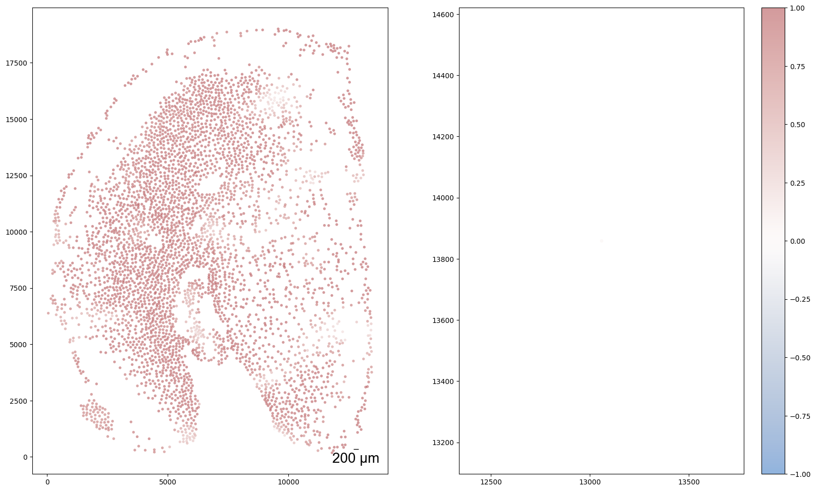
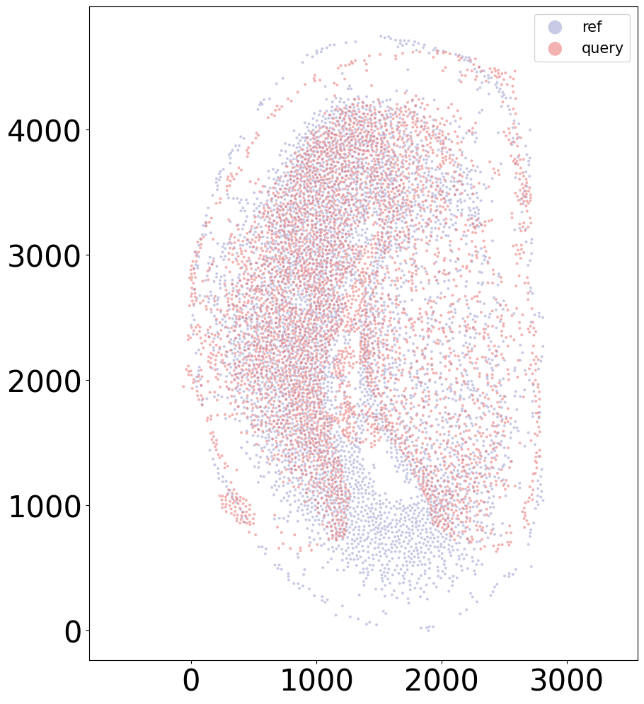
coords_final = CAST_STACK(coords_raw, embed_dict, stack_outdir, graph_list, params_dist, rescale=True)
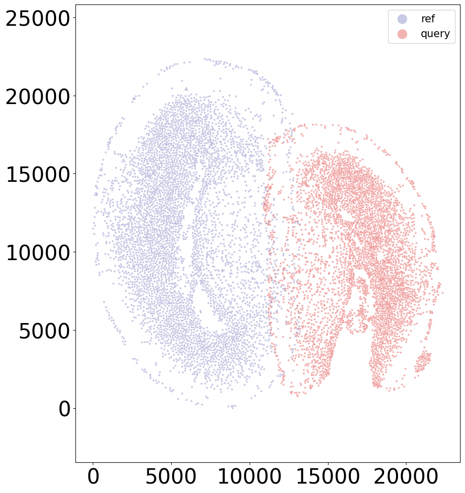
Aligning the left and right hemispheres of specific samples
[11]:
### List of samples
print(list(coords_raw.keys()))
['20DPI_3_left', '20DPI_3_right', '5DPI_3_right', '5DPI_3_left', '10DPI_3_left', '10DPI_3_right', '2DPI_3_left', '2DPI_3_right', '10DPI_1_left', '10DPI_1_right', '20DPI_2_left', '20DPI_2_right', '60DPI_right', '60DPI_left', '2DPI_2_left', '2DPI_2_right', '5DPI_2_left', '5DPI_2_right', '5DPI_1_left', '5DPI_1_right', '15DPI_1_right', '15DPI_1_left', '15DPI_4_right', '15DPI_4_left', '30DPI_right', '30DPI_left', '15DPI_3_right', '15DPI_3_left', '20DPI_1_left', '20DPI_1_right', '10DPI_2_right', '10DPI_2_left', '15DPI_2_right', '15DPI_2_left', '2DPI_1_right', '2DPI_1_left', 'Control_Juv_left', 'Control_Juv_right']
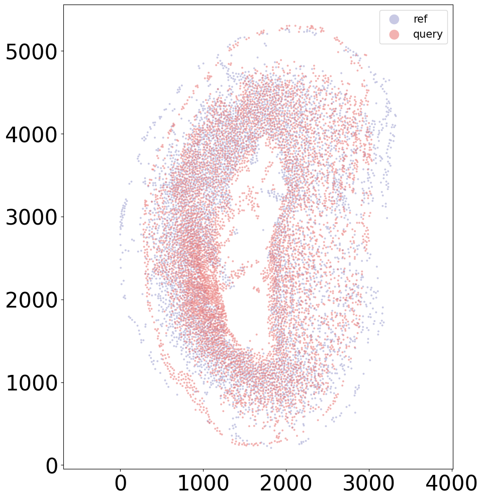
[12]:
sample = '20DPI_3'
align(f"{sample}_left", f"{sample}_right", 'demo7')
Loss: 930.137: 100%|██████████████████████████| 300/300 [00:04<00:00, 61.12it/s]
Loss: 504.696: 100%|██████████████████████████| 160/160 [00:11<00:00, 13.48it/s]
100%|████████████████████████████████████████| 160/160 [00:01<00:00, 124.46it/s]

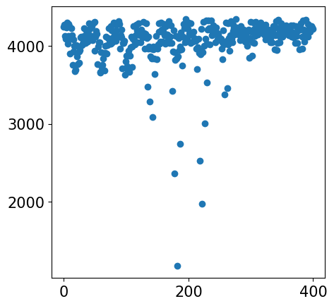
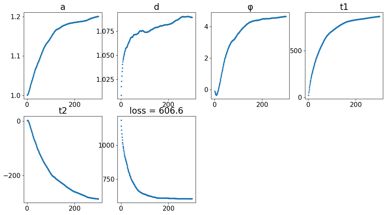
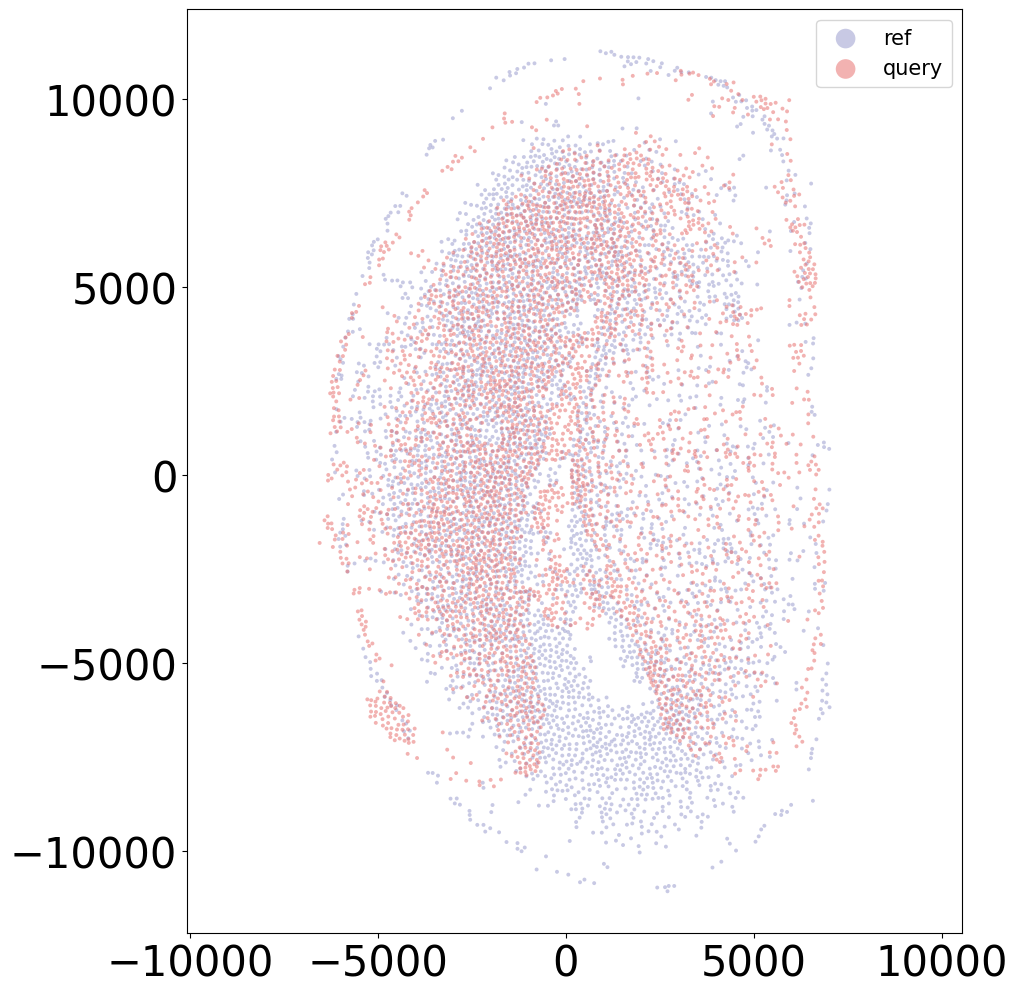
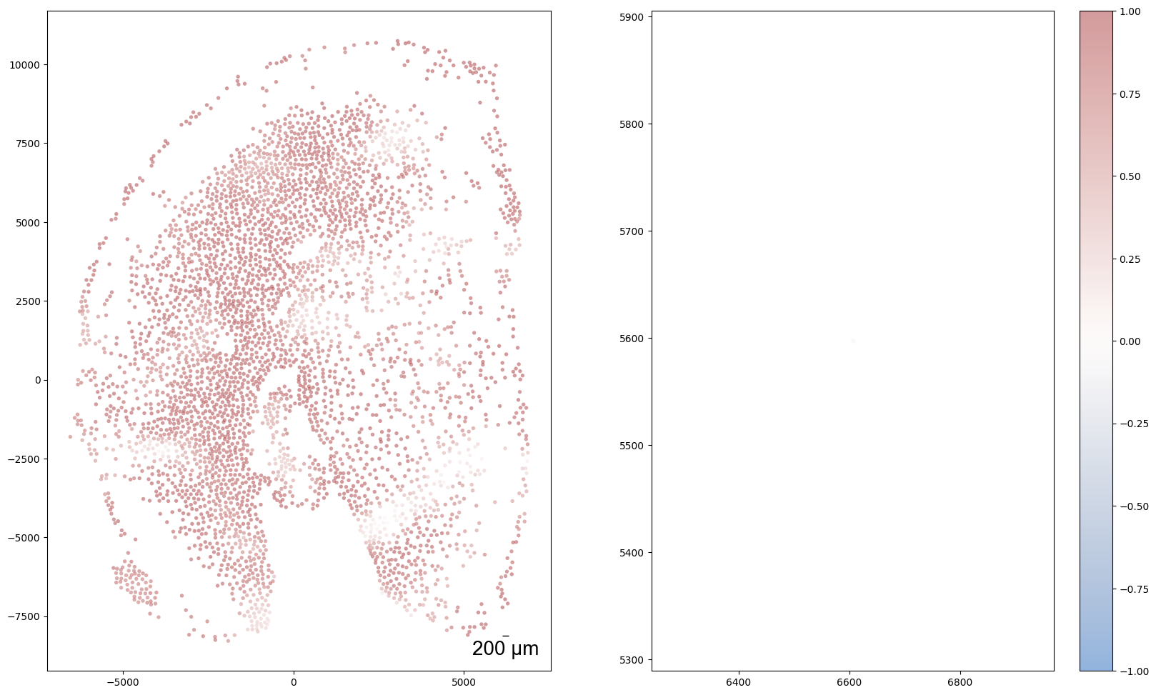
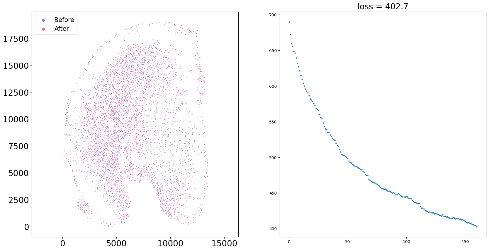
[13]:
sample = '2DPI_3'
align(f"{sample}_left", f"{sample}_right", 'demo7')
Loss: 606.580: 100%|██████████████████████████| 300/300 [00:03<00:00, 77.60it/s]
Loss: 402.671: 100%|██████████████████████████| 160/160 [00:11<00:00, 13.82it/s]
100%|████████████████████████████████████████| 160/160 [00:01<00:00, 126.69it/s]
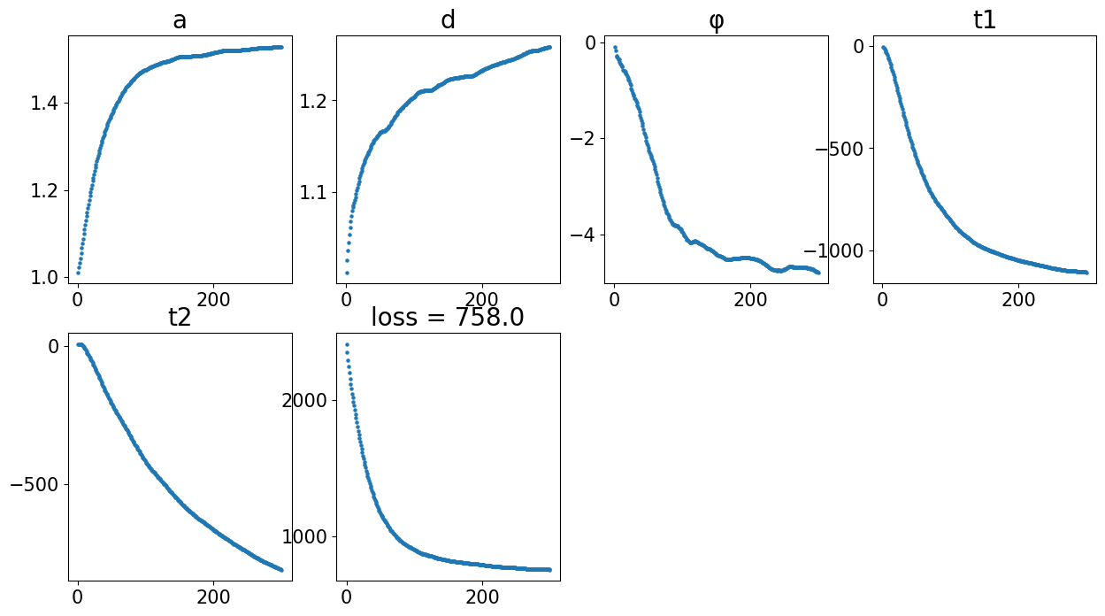
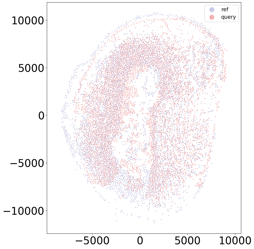
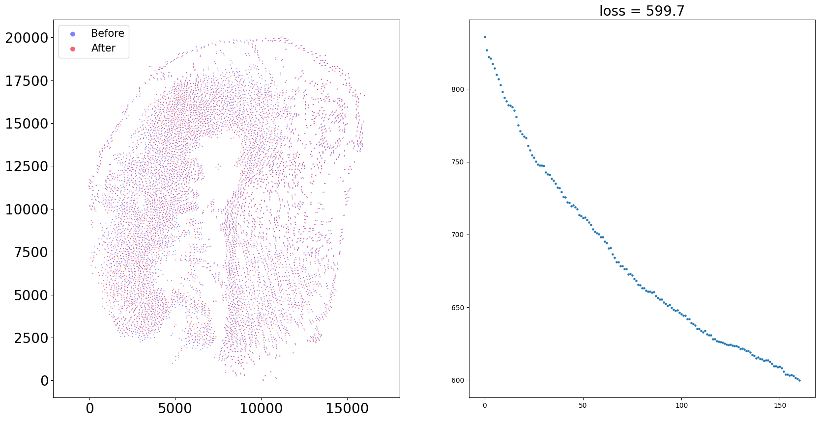
[14]:
sample = '15DPI_1'
align(f"{sample}_left", f"{sample}_right", 'demo7')
Loss: 758.042: 100%|██████████████████████████| 300/300 [00:03<00:00, 75.57it/s]
Loss: 599.721: 100%|██████████████████████████| 160/160 [00:11<00:00, 13.77it/s]
100%|████████████████████████████████████████| 160/160 [00:01<00:00, 126.37it/s]
Aligning the left and right hemisphere of all samples
[15]:
for sample in adata.obs['sample'].unique():
    print(sample)
    align(sample + '_left', sample + '_right', 'demo7')
    plt.close('all')
20DPI_3
Loss: 930.137: 100%|██████████████████████████| 300/300 [00:04<00:00, 61.63it/s]
Loss: 504.696: 100%|██████████████████████████| 160/160 [00:11<00:00, 13.38it/s]
100%|████████████████████████████████████████| 160/160 [00:01<00:00, 126.12it/s]
5DPI_3
Loss: 796.851: 100%|██████████████████████████| 300/300 [00:03<00:00, 79.20it/s]
Loss: 517.924: 100%|██████████████████████████| 160/160 [00:11<00:00, 14.24it/s]
100%|████████████████████████████████████████| 160/160 [00:01<00:00, 124.39it/s]
10DPI_3
Loss: 715.430: 100%|██████████████████████████| 300/300 [00:04<00:00, 67.83it/s]
Loss: 510.926: 100%|██████████████████████████| 160/160 [00:11<00:00, 13.64it/s]
100%|████████████████████████████████████████| 160/160 [00:01<00:00, 125.11it/s]
2DPI_3
Loss: 606.580: 100%|██████████████████████████| 300/300 [00:03<00:00, 78.08it/s]
Loss: 402.671: 100%|██████████████████████████| 160/160 [00:11<00:00, 13.83it/s]
100%|████████████████████████████████████████| 160/160 [00:01<00:00, 125.16it/s]
10DPI_1
Loss: 994.897: 100%|██████████████████████████| 300/300 [00:04<00:00, 71.10it/s]
Loss: 301.393: 100%|██████████████████████████| 160/160 [00:11<00:00, 13.64it/s]
100%|████████████████████████████████████████| 160/160 [00:01<00:00, 124.63it/s]
20DPI_2
Loss: 1243.203: 100%|█████████████████████████| 300/300 [00:05<00:00, 59.38it/s]
Loss: 288.493: 100%|██████████████████████████| 160/160 [00:11<00:00, 13.52it/s]
100%|████████████████████████████████████████| 160/160 [00:01<00:00, 125.68it/s]
60DPI
Loss: 662.997: 100%|██████████████████████████| 300/300 [00:04<00:00, 61.60it/s]
Loss: 374.864: 100%|██████████████████████████| 160/160 [00:11<00:00, 13.46it/s]
100%|████████████████████████████████████████| 160/160 [00:01<00:00, 123.63it/s]
2DPI_2
Loss: 619.750: 100%|██████████████████████████| 300/300 [00:03<00:00, 80.83it/s]
Loss: 304.291: 100%|██████████████████████████| 160/160 [00:11<00:00, 13.79it/s]
100%|████████████████████████████████████████| 160/160 [00:01<00:00, 125.75it/s]
5DPI_2
Loss: 1049.427: 100%|█████████████████████████| 300/300 [00:03<00:00, 77.56it/s]
Loss: 612.987: 100%|██████████████████████████| 160/160 [00:11<00:00, 14.43it/s]
100%|████████████████████████████████████████| 160/160 [00:01<00:00, 123.98it/s]
5DPI_1
Loss: 1092.192: 100%|█████████████████████████| 300/300 [00:03<00:00, 78.69it/s]
Loss: 595.907: 100%|██████████████████████████| 160/160 [00:11<00:00, 13.91it/s]
100%|████████████████████████████████████████| 160/160 [00:01<00:00, 127.11it/s]
15DPI_1
Loss: 758.042: 100%|██████████████████████████| 300/300 [00:03<00:00, 75.21it/s]
Loss: 599.721: 100%|██████████████████████████| 160/160 [00:11<00:00, 13.80it/s]
100%|████████████████████████████████████████| 160/160 [00:01<00:00, 127.10it/s]
15DPI_4
Loss: 874.195: 100%|██████████████████████████| 300/300 [00:04<00:00, 61.47it/s]
Loss: 510.448: 100%|██████████████████████████| 160/160 [00:12<00:00, 13.25it/s]
100%|████████████████████████████████████████| 160/160 [00:01<00:00, 126.19it/s]
30DPI
Loss: 577.515: 100%|██████████████████████████| 300/300 [00:04<00:00, 71.18it/s]
Loss: 343.533: 100%|██████████████████████████| 160/160 [00:11<00:00, 13.70it/s]
100%|████████████████████████████████████████| 160/160 [00:01<00:00, 124.38it/s]
15DPI_3
Loss: 921.260: 100%|██████████████████████████| 300/300 [00:04<00:00, 69.67it/s]
Loss: 454.544: 100%|██████████████████████████| 160/160 [00:11<00:00, 13.73it/s]
100%|████████████████████████████████████████| 160/160 [00:01<00:00, 123.75it/s]
20DPI_1
Loss: 1031.434: 100%|█████████████████████████| 300/300 [00:04<00:00, 65.21it/s]
Loss: 471.317: 100%|██████████████████████████| 160/160 [00:11<00:00, 13.56it/s]
100%|████████████████████████████████████████| 160/160 [00:01<00:00, 119.68it/s]
10DPI_2
Loss: 1198.918: 100%|█████████████████████████| 300/300 [00:04<00:00, 67.61it/s]
Loss: 583.949: 100%|██████████████████████████| 160/160 [00:11<00:00, 13.46it/s]
100%|████████████████████████████████████████| 160/160 [00:01<00:00, 124.63it/s]
15DPI_2
Loss: 1079.317: 100%|█████████████████████████| 300/300 [00:04<00:00, 67.51it/s]
Loss: 472.226: 100%|██████████████████████████| 160/160 [00:11<00:00, 13.43it/s]
100%|████████████████████████████████████████| 160/160 [00:01<00:00, 123.48it/s]
2DPI_1
Loss: 558.298: 100%|██████████████████████████| 300/300 [00:03<00:00, 84.60it/s]
Loss: 415.150: 100%|██████████████████████████| 160/160 [00:11<00:00, 13.96it/s]
100%|████████████████████████████████████████| 160/160 [00:01<00:00, 125.69it/s]
Control_Juv
Loss: 784.191: 100%|██████████████████████████| 300/300 [00:05<00:00, 56.90it/s]
Loss: 279.450: 100%|██████████████████████████| 160/160 [00:12<00:00, 12.97it/s]
100%|████████████████████████████████████████| 160/160 [00:01<00:00, 126.39it/s]